Gradient Descent for Linear Regression from Scratch

Introduction

Gradient descent (GD) is an optimization algorithm used in machine learning to find the best parameters that minimize the loss by finding the minima of the function. The algorithm is explained in detail in this gradient descent blog.

Gradient descent is a fundamental concept in the machine-learning field and is widely adopted to obtain optimal parameters. In this blog, we will see how gradient descent is implemented from scratch for a linear regression algorithm to find the optimal parameters w and b.

Linear Regression

Linear regression is an algorithm that finds the best line/plane that best fits the given data. Following is the geometric interpretation of linear regression.

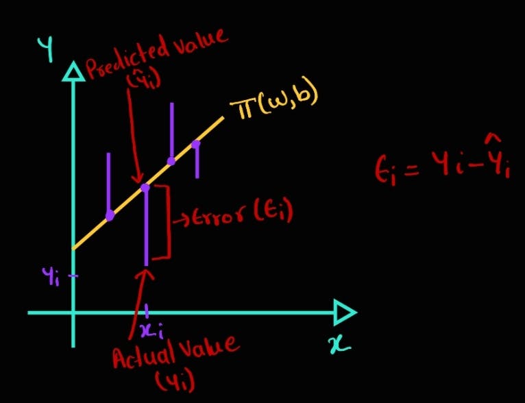
$$ y = f(x) = w^T*x + b$$

The error obtained for a given input xi is as follows:

$$e_i = y_i - \hat y_i$$

To get the best-fit line, the sum of all the errors must be minimized across the training data as follows:

$$min \sum_{i} error_i$$

Some errors might be positive and some may be negative, and there is a possibility that they might cancel each other. To avoid this, we take the sum of squares of errors.

$$min \sum_{i}(error_i)^2= min\sum_{i}(y_i-\hat y_i)^2$$

The loss function that must be optimized to find the best parameters of linear regression is as follows:

$$(w^*,b^*)= argmin_{w,b} \sum_{i=1}^{N}(y_i - (w^Tx_i +b))^2$$

Implementing GD for the above Loss Function

import libraries and initialize x, y


import numpy as np

# initialize x and y
x = np.random.randn(10,1)
y = 6*x + np.random.rand()

Initialize the parameters and set the hyperparameter learning rate

  # initialize x and y
  x = np.random.randn(10,1)
  y = 6*x + np.random.rand()

  # initialize parameters (w, b)
  w = np.random.rand(1)[0]
  b = np.random.rand(1)[0]

  # learning rate
  lr = 0.01

Write the logic for gradient descent

# gradient descent logic
def grad_desc(x,y,w,b,lr):
    # initialize gradient values
    dl_dw = 0
    dl_db = 0
    N = x.shape[0]
    for xi, yi in zip(x, y):
        # partial derivatives
        dl_dw += -2 * xi * (yi - (w*xi +b))
        dl_db += -2 * (yi - (w*xi +b))

    # update equation
    w = w - lr * dl_dw * 1/N
    b = b - lr * dl_db * 1/N

    return w, b

Update the gradient descent equation at each epoch to find the best parameters

  # update 
  def update(epochs,x,y,w,b,lr):
      for epoch in range(epochs):
          w, b = grad_desc(x,y,w,b,lr)
          yhat = (w*x)+b
          loss = np.divide(np.sum((y - yhat)**2, axis=0), x.shape[0])
          if loss < 0.0001:
              print(f"minima is found at {epoch}th epoch and has loss of {loss}")
              print(f"optimal parameters are w:{w}, b:{b}")
              break

Run the code and find the optimal parameters that minimize the loss function

update(50000,x,y,w,b,lr)

The output obtained is as follows:

minima is found at 386th epoch and has loss of [9.81000523e-05]
optimal parameters are w:[5.98897974], b:[0.49323804]

Conclusion

Gradient descent is a simple yet powerful algorithm used for optimisation. Also, it is very simple to implement as we saw in this article. The beauty of the algorithm is that we start with some random values for the parameters and at the end we get the optimal values of the parameters.

With some minor changes in the above code, stochastic gradient descent which is a variant of gradient descent can be implemented. This can reduce the number of computations required to find the minima.

Gradient Descent for Linear Regression from Scratch

Lets find the best parameters for linear regression using gradient descent optimisation.

Introduction

Linear Regression

Implementing GD for the above Loss Function

Conclusion