Introduction

Machine learning models learn by minimizing the loss at each iteration. The loss is the difference between the actual value and the value predicted by the model. This is achieved by finding the minima of the loss function. But what is minima and how to find it?

Minima is the smallest value taken by the function in a given range (Local minima) or within the entire domain of the function (global minima). The slope at the minima is zero. Minima is calculated by taking the derivative of the function and equating it to zero. Solving this equation will give the value of minima.

Gradient descent is an optimization algorithm which is widely adopted by the machine learning community for minimizing loss function and finding the best parameters for the models. But why do we need an algorithm when we can just find the derivative of the function and equate it to zero? The following section will answer the question.

Why do we need Gradient Descent?

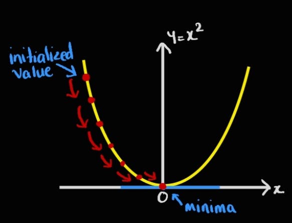
Let us consider a simple square function and find minima for it as shown below. We can easily find the derivative of the square and find the minima value. The minima value occurs at x=0.

If finding minima using this method is so simple then why can't we use this method for finding the best parameters of models? In the real-world scenario, the function can be very complex and multivariate. Finding minima in such cases using the analytical approach or using linear algebra can become complex.

Hence, we need an algorithm to reduce the loss of this complex function and find the minima. The gradient descent algorithm iteratively reduces the loss till convergence i.e. reaching the minimum point of a highly complex function.

How does Gradient Descent work?

In Gradient descent, the update equation at every iteration is given as follows:

$$x_i = x_{i-1} + \eta *(-\frac{df}{dy})_{x_{i-1}}$$

$$Where,\space x_i=new \space value,\space x_{i-1}=old \space value,\space \eta= Learning \space rate$$

Algorithm

• Pick an initial value x0 at random.

• Compute x1 using the gradient descent update equation. If the slope at x1 is positive then x1 < x0. Else if the slope is negative, then x1> x0.

$$x_1 = x_0 + \eta *(-\frac{df}{dy})_{x_0}$$

• Similarly, compute x2, x3 , .........., x_k-1, x_k

$$Where, x_k = x_{k-1} + \eta *(-\frac{df}{dy})_{x_{k-1}}$$

• Continue the loop till (x_k - x_k-1) is very very small. This is the point of convergence and we terminate the loop at this stage and declare x* = x_k as minima.

Note: If the function is multivariate, then we would have to calculate the partial derivate of a function w.r.t each variable and compute an update equation for each variable simultaneously at each iteration.

Learning Rate

The learning rate is denoted as eta in the update equation and controls the rate at which gradient update or learn the parameters of the model. The learning rate is a hyperparameter and should be tuned properly.

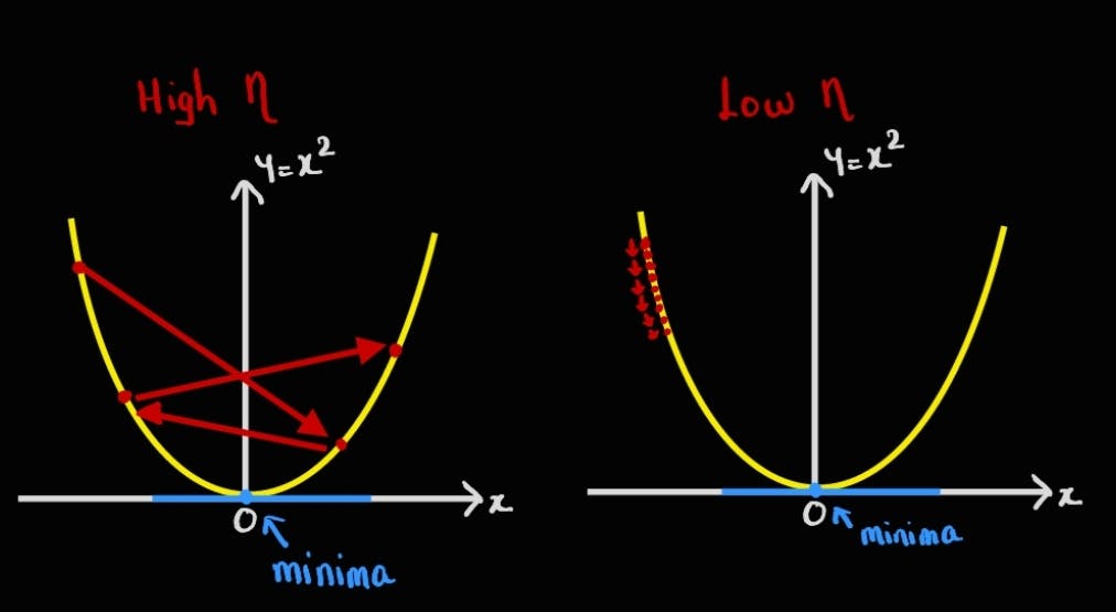
As seen from the above images, if:

• the learning rate is too high, then there are chances of overshooting and missing the minima value. This could lead to not reaching to minima value ever.

• the learning rate is very low, updates at iterations are small and it would take a very long time for convergence.

Can it be improved further?

If the number of data points in the dataset is large, then gradient descent takes lots of time for convergence and becomes computationally expensive. How do we tackle this situation?

• Stochastic gradient descent (SGD) can be used to overcome the issue.

• In SGD, instead of using all the data points at each iteration for updation, it uses randomly selected k points and performs the same update for multiple iterations.

• After some iterations, the x* obtained by SGD will be the same as the x* obtained by GD.

At each iteration set of random points chosen are different. Suppose there are n data points, if:

• K=1, the algorithm is called SGD.

• K>1, it is Batch SGD.

• K=n, then SGD becomes GD.

The number of iterations required in SGD is more compared to GD, but convergence time is faster due to the lesser number of points at each iteration. And results obtained by SGD are similar to that of GD.

Conclusion

• Gradient descent is an iterative algorithm used to optimize the machine learning models and to find the best parameters for the model.

• It can optimize highly complex functions and find the minima.

• The learning rate must be tuned properly to reach the point of convergence efficiently.

• The algorithm can be further improved by using batches of data for updation, and the algorithm is called stochastic gradient descent.